Nowadays, analytical solutions are becoming mission critical
for many organizations. Microsoft SQL Server 2008 Analysis Services
(SSAS) is designed to provide exceptional performance and scalable support
with millions of records and thousands of users from different locations.
Why to Build a
Cube?
There are many advantages of cube over
relational data mart.
- While querying a data mart, you
can get most of the results but not everything you need for business
analysis and decision making. Cube can help you to get answers
of all "What-If" scenarios.
- Building a cube helps to house
your data to centralize the business rules for calculations that you can't
easily store in a relational data mart.
- The structure of the cube makes it
much easier to write queries to compare data year over year (YOY), or to
create cumulative values such as year-to-date (YTD) sales.
- Scalable Infrastructure - Analysis
Services can scale to support databases of many terabytes in size with
many thousands of users.
- Superior Performance - Analysis
Services cubes are multidimensional structures that enable fast access to
high volumes of pre-aggregated data, empowering end users to gain insight
into relevant business data at the speed of thought.
- You gain the ability to manage
aggregated data in the cube. To improve query performance in a relational
data mart, we often create summary tables to prepare data for queries that
don't require transaction-level detail. SSAS creates the logical
equivalent of summary tables (called aggregations) and keeps them
up-to-date.
Creating a Cube consists of the following steps:
- Creating Analysis Services Project
- Creating Data Source
- Creating Data Source View
- Creating Cube and Dimensions
- Creating Dimension Hierarchies
- Deploying Cube Database from BIDS
First step is to create a project in
Business Intelligence Development Studio (BIDS). Launch BIDS from Start --> All
Programs --> Microsoft SQL Server
2008 --> SQL Server Business Intelligence
Development Studio and then click File
--> New --> Project.
In the New Project dialog box, select Analysis
Services Project. In the Name text box, type MYSSASFirstProject and,
if you like, change the location for your project. I'll store this
project at location D:\SSASProjects. Click OK to create the
project.
Now add a data source to define the connection
string for data mart AdventureWorksDW2008R2. In Solution Explorer,
right-click the Data Sources folder and click New
Data Source.
In the Data Source Wizard, click
Next on the Welcome to the Data
Source Wizard page if it hasn't
been disabled. On the Select how to define the
connection page, click New to set up a new
connection. In the Connection Manager, the default provider is the Native
OLE DB\SQL Server Native Client 10.0, which
is correct for our project.
To define the connection,
type the name of your server in the Server
Name text box. Alternatively you can select it from
the drop-down list, then select AdventureWorksDW2008R2 in the database drop-down list and click Test Connection button
to check the connection. Finally click on OK as shown below:
When you're back in the Data Source Wizard, click Next. On the Impersonation Information page, select Use the service account option so that service
account will be used to read data from the source when loading data
into your SSAS database and service account must have read
permissions to do so. Click Next and then Finish to complete the wizard.
Now next step is to create a data source view (DSV) from the data source to
define dimensions and cubes. You can make changes to the DSV without modifying
the actual data source, which is very useful if you have only read permissions
to the data mart. In Solution Explorer,
right-click on the Data Source Views
folder and then click New Data Source Views...You
can see Data Source View Wizard. Click Next on the Welcome page. On the Select a Data Source page, select the data source
just added to the project (Adventure Works DW2008R2.ds) and click Next. Now
add required objects to the DSV by double-clicking each table or view on Select Tables and Views page. I want to add
the following tables to the DSV to make it easy to understand for beginners:
DimDate,
DimProduct, DimProductCategory,
DimProductSubcategory, and FactInternetSales. You can always add more
tables later if you want to explore advance BI questions. Now click Next in the
Data Source View Wizard once you are finished adding required tables followed
by click on Finish. You can give a name to your DSV before
clicking Finish
button.
I would recommend you to change the
name of objects by selecting each one in the DSV designer and remove the Dim and Fact
prefixes from the FriendlyName
property because when you create dimensions and cubes, only
FriendlyName property will be assigned to the objects.
The DSV is shown below:
Next step is to create a Cube and Dimensions from the data
source view. In Solution Explorer, right-click on the Cubes folder and then click New Cube...You can see Cube Wizard. Click on Next in Welcome to the Cube Wizard page.On the Select Creation Method page, keep the default
option Use
existing tables and click Next button. On the Select
Measure Group Tables page, choose InternetSales table and
click Next.
Now the wizard displays all the measures
available in the selected measure group tables. Measures are basically numeric
values e.g. OrderQuantity, Unit Price, Sales Amount, Tax Amount etc. Select
only the following measures from Internet Sales Group: Order Quantity, Unit
Price, Total Product Cost, Sales Amount, and Internet
Sales Count
Now click on Next button to open Select
New Dimensions page and select Date and Product dimensions. Click Next to
proceed.
In the Completing the Wizard
page, enter the cube name as AdventureWorksCube and click Finish
button to complete the wizard. Cube layout is shown below:
Now click on each dimensions and add required attributes
from the Data Source View.
Date Dimension:
Drag and drop FullDateAlternateKey, CalendarYear,
CalendarQuarter, EnglishMonthName, and EnglishDayNameOfWeek. Rename
FullDateAlternateKey with Full Date, EnglishMonthName with Calendar Month, and
EnglishDayNameOfWeek with Calendar Week as shown below:
Product Dimension:
Drag and drop EnglishProductCategoryName from
ProductCategory table, EnglishProductSubcategoryName from ProductSubcategory
table and Color, ModelName, Size and Weight from Product table.
Navigate to Date Dimension Structure. Drag and drop Calendar Year attribute into Hierarchies surface
area following by Calendar Quarter, Calendar Month,
Calendar Week , and Full Date attributes.
Rename hierarchy with Calendar. You'll see a warning
mark in the hierarchy because attribute relationship is not set properly.
Set Attribute Relationships
Click on the Attribute
Relationships tab in the dimension designer. This tab is available
only in Analysis Services 2008. By default, all attributes relate directly
to the key attribute, Date Key as shown
below:
To optimize the design by reassigning relationships, Right
Click on Full Date and select New
Attribute Relationship. Select Related
Attribute as Calendar Week and Relationship type as Rigid
(will not change over time). Repeat same
thing for remaining attributes. Finally Attribute Relation will look like below
image:
Now it’s time to deploy the cube at required
server. Right click on the project (MYSSASFirstProject in this example) and click properties to open project properties
page. Enter Server Name name Server property and Database name in Database
property as shown below:
Click OK to save changes. Now right click on the
project and click on Process to Build and Deploy the project. You will a
message while deploying the database first time.
Click on Yes to proceed. Now you can see Process
Database - PreojectName window. Click on Run to continue.
Once the database is deployed and processed successfully,
you can see the data through Browser tab or directly through SQL Server
Analysis Services. You can also pull cube data in Excel using Excel OLAP Pivot
Tables, which is the preferred option used by business managers.
Structure of Cube
In Cube Designer, you can
view and edit various properties of a cube. The designer contains the following
tabs, which display different views of the cube.
Use this tab to modify the
architecture of a cube.
Use this tab to define the
relationships between dimensions and measure groups, and the granularity of
each dimension within each measure group. If you use multiple fact tables, you
might have to identify whether measures do not apply to one or more dimensions.
Each cell represents a potential relationship between the intersecting measure
group and dimension.
Use this tab to examine
calculations that are defined for the cube, to define new calculations for the
whole cube or for a subcube, to reorder existing calculations, and to debug
calculations step by step by using breakpoints. Calculations let you define new
members and measures based on existing values, such as a profit calculation,
and to define named sets.
Use this tab to create,
edit, and modify the Key Performance Indicators (KPIs) in a cube. KPIs enable
the designer to quickly determine useful information about a value, such as
whether the defined value exceeds a goal or falls short of the goal, or whether
the trend for the defined value is getting better or worse.
Use this tab to create or
modify drill through, reporting, and other actions for the selected cube.
Actions provide to client applications context-sensitive information, commands,
and reports that end users can access.
Use this tab to create and
manage the partitions for a cube. Partitions let you store sections of a cube
in different locations with different properties, such as aggregation
definitions.
Use this tab to create and
manage the perspectives in a cube. A perspective is a defined subset of a cube,
and is used to reduce the perceived complexity of a cube to the business user.
Use
this tab to create and manage translated names for cube objects, such as month
or product names.
Use
this tab to view data in the cube.
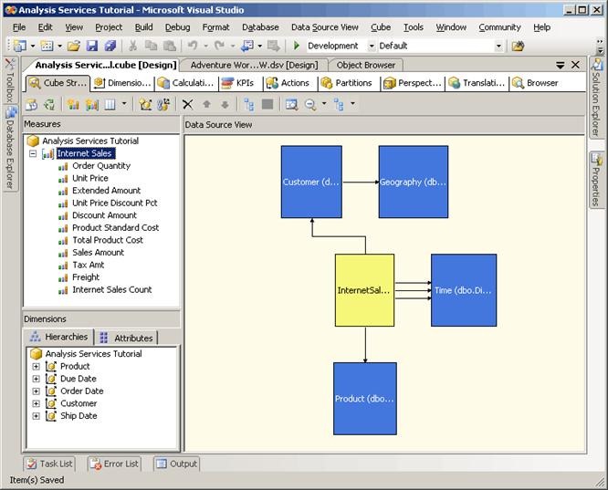
In
the Measures pane of the Cube Structure tab in Cube Designer,
expand the Internet Sales measure group.
The
measures that are defined for the Internet Sales measure group appear. You can
change the order of these measures by dragging the measures into the order that
you want. The order will affect how certain client applications order these
measures. The measure group is named Internet Sales because the underlying fact
table had the friendly name of InternetSales in the data source view. Notice
that a space was added automatically, based on the capitalized letter
"S", to increase the user-friendliness of the name. The measure group
and each measure that it contains have properties that you can edit in the
Properties window.
The
following image shows the measure group and measures in the Measures
pane of Cube Designer.
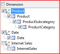
In
the Dimensions pane of the Cube Structure tab in Cube Designer,
review the cube dimensions that are in the Analysis Services Tutorial cube.
Notice
that while only three dimensions were created at the database level, as
displayed in Solution Explorer, there are five cube dimensions in the Analysis
Services Tutorial cube. The cube contains more dimensions than the database
because the Time database dimension is used as the basis for three separate
time-related cube dimensions, based on different time-related facts in the fact
table. These time-related dimensions are also called role playing dimensions.
The three time-related cube dimensions let users dimension the cube by three
separate facts that are related to each product sale:
The
product order date, the due date for fulfillment of the order, and the ship
date for the order.
By
reusing a single database dimension for multiple cube dimensions, Analysis
Services simplifies dimension management, uses less disk space, and reduces overall
processing time.
3.
In the Dimensions pane of the Cube Structure tab, expand Customer,
and then click Edit Customer.
The
Customer dimension appears in Dimension Designer. (Note that Data Source View
Designer and Cube Designer remain open.) Dimension Designer contains three
tabs: Dimension Structure, Translations, and Browser.
Notice that the Dimension Structure tab includes three panes: Attributes,
Hierarchies and Levels, and Data Source View. The attributes that
the Cube Wizard designed appear in the Attributes pane and the user
hierarchy that the Cube Wizard defined appears in the Hierarchies and Levels
pane. The Data Source View pane displays the tables in the data source
view from which columns are used as attributes in this dimension.
You
add, remove, and edit hierarchies, levels, and attributes on the Dimension
Structure tab of Dimension Designer.
The
following image shows the Dimension Structure tab of Dimension Designer.
4.
Switch to Cube Designer by clicking the tab in the design environment or by
right-clicking the Analysis Services Tutorial cube in the Cubes node in
Solution Explorer and then clicking View Designer.
5.
In Cube Designer, click the Dimension Usage tab.
In
this view of the Analysis Services Tutorial cube, you can see the cube
dimensions that are used by the Internet Sales measure group. When a cube has
multiple measure groups, cube dimensions might be used with some measure groups
but not with others. Also, you define the type of relationship between each
dimension and each measure group in which it is used.
The
following image shows the Dimension Usage tab of Cube Designer.
6.
Click the Customer field next to Customer at the intersection of
the Internet Sales measure group and the Customer dimension, and then click the
ellipsis button (…).
The
Define Relationship dialog box appears. In this dialog box, you define
the custom dimension properties within a specific measure group. By default,
dimensions have the same behavior in each measure group. However, they can have
different behavior in different measure groups. Notice that the relationship of
the Customer dimension to the Internet Sales measure group is a Regular
relationship, which means that the DimCustomer dimension table is directly
joined to the FactInternetSales measure group table. Notice also that the granularity
of this dimension is at the lowest level, namely the Customer level, but that
you can define different levels of granularity. In Lesson 5, you will learn
about defining a custom granularity level.
The
following image shows the Define Relationships dialog box.
7.
Click Advanced.
The
Measure Group Bindings dialog box appears, which lets you change the
binding of each attribute and define null processing settings. The binding for
an attribute specifies the column in the underlying dimension table to which
the attribute is bound. By default, this setting is inherited from the
dimension; this setting is rarely changed at the measure group level. Null
processing settings let you define how Analysis Services treats null values
during processing at the measure group level; these settings override any
settings at the dimension level.
The
following image shows the Measure Group Bindings dialog box.
8.
Click Cancel, and then click Cancel again, to return to Cube
Designer.
Introduction
if reporting access to cubes can be provided from Microsoft Excel, then report
building can be performed by an end user. Majority of the time, using this
method, users can construct reports the way they wish. Improvements in
Excel 2007 have provided a number of new fancy features that can be
used with cubes.
Connecting to
SSAS using Microsoft Excel
Launch Microsoft
Excel first. Select the option, select the Data table, then select the From
Other Services button in the Data ribbon, and then select From Analysis
Services. As shown in Figure 2, a list of available data sources is provided.
In the Analysis Services option is the screen shown below. To connect to the
SSAS servers, login credentials need to be provided. However, SSAS does not
support SQL Server authentication, hence the Windows Authentication option must
be selected.
After providing the login credentials, the SSAS database and the Cube need to be
selected as shown below.
All cubes for the selected SSAS database will be listed. Only one cube can be
specified at this point. The next step is to set the configurations to
the Data connection file. There are options to specify the file name and the
path for the Data connection file.
Next select sheet whether a Report or chart is wanted.
Viewing
Data
now are the most fascinating steps, viewing the SSAS data from an Excel
file. In the right side of the excel sheet, notice a PivotTable Field
List. Within this list the KPI, measures and dimension attributes can be
seen; the user is able to select the attributes they want.
To see the Sales
amount for each product color and class.; simply select Class and Color from
the Product dimension and Sales Amount.
A pivot table can be designed with columns and row headers as shown in below.


